Applying Control Theory: Interpret Bode Diagrams
Discussions about hydro-mechanical system dynamics make it clear that component selection and system design have tremendous impact on system performance and stability. Although advanced mathematics and modern computer programs have provided methods for accurate assessment of system design elements, it is often (usually) not feasible, or necessary, to use more than a simple set of assumptions and tools to reach a reasonable approximation of system performance from which to begin further refinement.
One of the more useful tools for this purpose is the Bode Plot. This is a graph of the amplitude and phase of the system’s sinusoidal response as a function of the frequency versus the input signal.
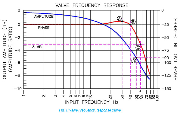
Fig. 1 shows an example of a Bode Diagram for a hydraulic servo valve. This type of plot makes it very straightforward to compare components and can also be used to analyze entire systems. There are several things to notice about this plot and each will be discussed in turn.
Input
The input to the valve was a fixed amplitude, sinusoidal current input to the servo valve torque motor. (This could also have been to the coils of a proportional valve.) The plot begins by plotting the output response to the fixed amplitude signal at 0 Hz and increasing the frequency of the input signal while controlling for constant amplitude.
Output
The output will be different from the input (flow versus current) and will attempt to follow the input. Thus, as the constant amplitude current signal to the valve increases in frequency, the valve will oscillate back and forth in an attempt to respond appropriately to the input signal. As the valve cycles, so, too, will the output.
Amplitude
Amplitude is always represented in decibels referenced to the input signal.

Amplitude expressed in dB (decibels)
Where:
On = Output at any frequency
Ol = Output at lowest frequency
Notice that the amplitude remains at 1 decibel as long as the valve spool is able to follow the input signal.
However, eventually a frequency will be reached where the valve’s phase lag will begin to deteriorate in its ability to maintain a one-to-one amplitude relationship to the input. That point is 40 Hz in Fig. 1. Notice how the output response falls from the frequency upward (point B).
Resonant Rise (Natural Frequency of the Valve)
What about the small rise in amplitude between 20Hz and 40Hz (point A)? Remember that every physical system (even this valve) has some natural frequency. The point at which, absent any damping, it will ring in response to an input. In the case of a hydro mechanical system, this resonance occurs as the result of the back-and-forth interaction between the potential energy stored in the capacitance elements of the system (compressible oil volume) and the kinetic energy of the moving mass. In this valve, there are additional resonance factors that involve the interaction between the spool and the electromechanical system making up the torque motor and flapper assembly.
When resonance occurs, it can manifest as a rise in the output amplitude at and around the resonant frequency and has been termed resonant rise. The existence of the 0.8dB rise above 0db around 30Hz indicates that this valve is slightly springy and that its output will tend to ring at roughly this frequency in response to a step input. This valve is underdamped. This springiness can be designed out of valves and, in this case, the valve will display no resonant rise and is said to be critically damped.
Attenuation is the reduced level of output as the valve is cycled at higher frequencies.
3dB Rolloff
3db Rolloff is a standardized logarithmic measure of how quickly a valve can change its output in response to a change in input command. More specifically, it is the input frequency that a valve’s amplitude decreases to -3dB of its peak attainable and useable value. Follow the Amplitude curve in Fig. 1. It reaches a point that as the input frequency increases, the curve crosses the -3dB line (point C). At that intersect, if a vertical line were drawn downward, the indicated input frequency for this valve is 57Hz.
For example, imagine an electro pneumatic regulator commanded to output a peak pressure of 15 PSI, and then sinusoidally commanded to 2 PSI then again to 15 PSI. If initially commanding at a low frequency, the 15 PSI peak pressure will be attainable. As the input frequency increases, however, the regulators ability to respond to the rapidly changing command will become more difficult. The regulator will no longer be able to achieve the 15 psi peaks. If the Bode plot in Fig. 1 were for this regulator, an input frequency at 57 Hz would only yield about 70% or approximately 10.5 PSI maximum peak pressure.
The -3dB Rolloff frequency is a common measure used to compare the performance of electro pneumatic and hydraulic valves. This value alone, however, does not allow for evaluation of how the valve will work with other components of the full system.
Phase Lag is the time required for a cyclic output to recreate a cyclic input (command). Phase lag is always represented in degrees.
90° Phase Lag
Turning to the phase plot of the output in Fig. 1, notice that the phase lag increases (as predicted) as the input frequency increases. Notice that the valve output is 90° behind the input at 50Hz (point D).
This frequency is termed the valve bandwidth and is the most useful metric for comparing valve performance. In addition to valve comparison, the 90° phase lag frequency is useful for assessing valve performance in the target system.
Bandwidth
The band of frequencies between 0Hz and a predetermined point on the frequency response curve characterize the frequency response of the valve. As noted previously, there are at least two common predefined points:
1. -3dB rolloff frequency is the frequency that the valve output is limited to 70% of its maximum
2. 90° phase lag frequency is the frequency that the valve output is 90° behind the valve input.
dB = 20 log (Δ output /Δ input)
= 20 log (70% / 100%)
= 20(-0.1549)
dB = -3.098
Depending upon which one is chosen, this valve’s bandwidth would be expressed as 55Hz or 50Hz, respectively.
Two additional valve criteria available on the Bode Plot are:
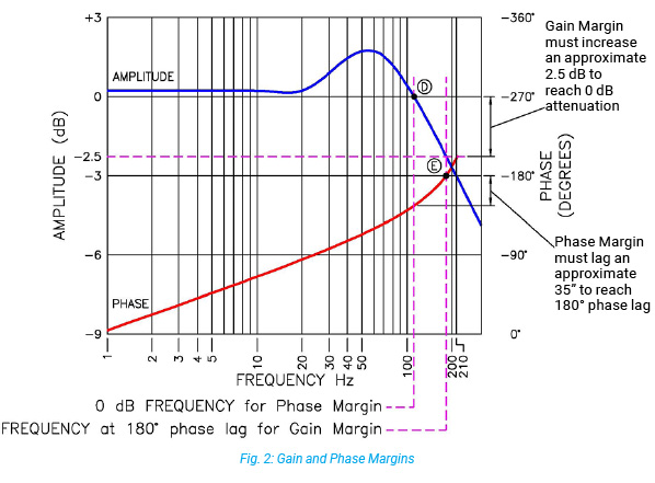
1. Phase Margin – is the amount by which the phase angle must additionally lag to reach 180 degrees phase lag when measured at the 0db frequency. It is a relative measure of system stability and is expressed in degrees. (35 degrees, point E in Fig. 2) As to not be limiting factor in system performance and stability, the natural frequency of the electro hydraulic valve is ideally two to three (or more) times the calculated natural frequency of the load ωL.
2. Gain Margin – this is the amount by which the loop gain must increase in order to achieve 0dB attenuation at the 180 degrees phase lag frequency of the Phase Margin, projected upward. It is a relative measure of system stability and is expressed in decibels. (2.5dB, point D in Fig. 2)
TEST YOUR SKILLS
In Fig. 2 what is the bandwidth as determined by referencing the 3dB rolloff?
a. 30Hz.
b. 190Hz.
c. 110Hz.
d. 210Hz.
e. 240Hz.
See the Solution
The correct answer is d.
Share this information.
Related Posts


One thought on “Applying Control Theory: Interpret Bode Diagrams”
Leave a Reply
Sponsor

Sponsors
Nice article !
One minor comment.
I believe on the Fig.1 the graph legends are reversed.
Amplitude should be labeled as phase and vice versa.